Data Table Excel

Click Insert PivotTable and then check Add this data to the Data Model in the Create PivotTable dialog box. With a table selected choose the Design tab on Excels ribbon and choose the Table Styles dropdown to add some style to your data.

20 Excel Table Tricks To Turbo Charge Your Data Pakaccountants Com Microsoft Excel Tutorial Excel Shortcuts Excel

Here are the steps to load this table in Excel.

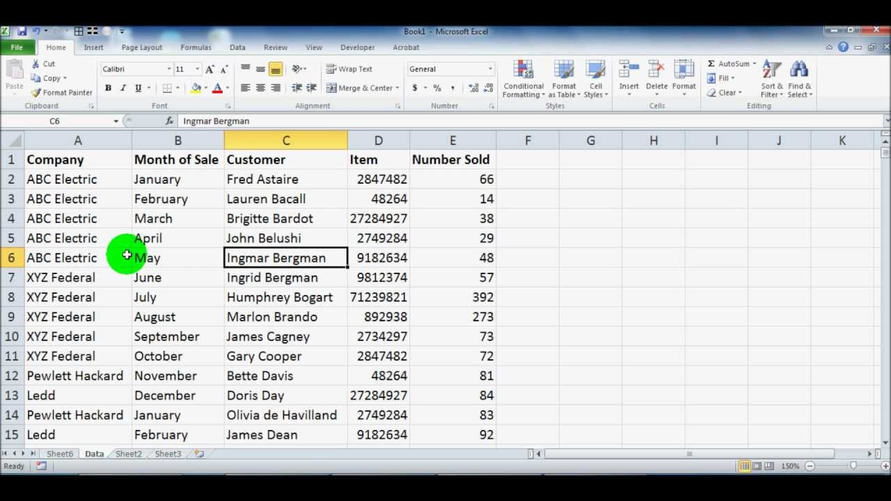
Data table excel. To create the table select any cell within the data range and press CtrlT. Click the File tab. Enhance Your Excel Skills With Expert-Led Online Video Courses - Learn Anywhere Anytime.

Excel will display the Create Pivot Table window. Select the data and in the Insert Tab under the excel tables Excel Tables In excel tables are a range with data in rows and columns and they expand when new data is inserted in the range in any new row or column in the table. Make sure the My table has headers box is checked and click.

Cell D4 on Sheet1 still appears to be and acts like the original input it replaces. Enhance Your Excel Skills With Expert-Led Online Video Courses - Learn Anywhere Anytime. To use a table click on the table and select the data range.

Sign Up for a 7-day Free Trial. 44 rows Click at the end of the Sample Data heading above the table you wont see anything. Use one of these approaches to add your data.

Click Power Pivot Add to Data Model. The following code filters a table myTable1 and referring to sheet1 of a rangeA1D10In this Case I am applying filter for second column and looking for description DDD in a table. Copy the sample data in the table above including the column headings and paste it into cell A1 of a new Excel worksheet.

Instead of spending time manually styling data you can use a table to clean up the look of your data. Create a new sheet select the cell A1 in the new sheet type this formula OFFSETmyrngROWSmyrng-ROWCOLUMNSmyrng-COLUMN myrng is the range name you give in step 1 press Shift Ctrl Enter keys and then drag the fill handle over cells to fill all the table data. If you only use tables to.

You can use ListObjectsTableNameRangeAutoFilter method for Filtering tables in excel VBA. For one variable data table the Row input cell is left empty and in a two-variable data table both Row input cell and Column input cell are filled. Cell E4 on Sheet1 is now the cell that drives all calculations throughout the model even though it appears to have been added.

To start off select any cell in the data and click Pivot Table on the Insert tab of the ribbon. Excel Data Tables are one of the What-if Analysis tools that we have available to aid our decision making. Start by selecting any cell within the data that you want to add to the model.

It is only useful when the formula depends on several values that can be used for two variables. Data Tables are one of Excels What If Analysis features. Read more section click on pivot tables.

It can be any range of data but data formatted as an Excel table is best. Things to Remember About Data Table in Excel. We can filter table in the following way.

With Excel Data Tables we can perform what-if analysis with one or two variables which makes it quick and easy to experiment and understand the outcome of different options. Instead of entering formulas and variables individually to compare results you can set up a Data Table with one or two variables. The default location for a new pivot table is New Worksheet.

Once the What-If analysis is performed and the values are calculated you cannot change or modify any cell from the set of values. Excel Data Tables. Ad Flexible Monthly Subscription Self-paced Online Course.

How to make a two way two variable data table in Excel - YouTube. Notice the data range is already filled in. Sign Up for a 7-day Free Trial.

The above steps would give you a table that has all the three tables merged Sales_Data table with one column for Pdt_Id and one for Region. Ad Flexible Monthly Subscription Self-paced Online Course. Click on Close and Load to.

They dont require knowledge of any new fancy formulas and are super quick to build. The Data Table links directly to a cell on the same sheet as the Data Table but indirectly to the input on the other worksheet. Data tables are used in Excel to display a range of outputs given a range of different inputs.

Two-Variable Data Table in Excel allows users to test two variables or values at one time or simultaneously in a data table for created formula. Compare Results in a Data Table. Create a Data Table With 1 Variable.

They are commonly used in financial modeling and analysis to assess a range of different possibilities for a company given uncertainty about what will happen in the future. In the Import Data dialog box select Table.

Excel Pivot Table

In the TableRange box type the range name. What is a pivot table.

Excel Pivot Tables Tutorial What Is A Pivot Table And How To Make One Pivot Table Microsoft Excel Tutorial Excel Shortcuts

A pivot table is a special Excel tool that allows you to summarize and explore data interactively.

Excel pivot table. A PivotTable is a powerful tool to calculate summarize and analyze data that lets you see comparisons patterns and trends in your data. Hence you can use the same steps to create a PivotTable form either a Range or Table. A Pivot Table is a tool in Microsoft Excel that allows you to quickly summarize huge datasets with a few clicks.

PivotTables work a little. A pivot table is a summary of your data packaged in a chart that lets you report on and explore trends based on your information. In the Grouping dialogue box select Years.

Select any cell in the Date column in the Pivot Table. You can use a PivotTable to summarize analyze explore and present summary data. Change your data set to a table before you insert a.

Join millions of learners from around the world already learning on Udemy. Notice the data range. Click any cell inside the pivot table.

Its a lot harder to explain a pivot table. Go to Pivot Table Tools Analyze Group Group Selection. Pivot tables are one of Excel s most powerful features.

A pivot table is a table that summarizes data in another table and is made by applying an operation such as sorting averaging or summing to data in the first. Join millions of learners from around the world already learning on Udemy. PivotCharts complement PivotTables by adding visualizations to the summary data in.

Pivot table in excel is used to categorize sort filter and summarize any length of data table which we want to get count sum values either in tabular form or in. On the Analyze tab in the Data group click Change Data Source. Excel will display the Create Pivot Table window.

Even if youre absolutely new to the world of Excel. Ad Learn Excel pivot tables with real-world case studies from a trusted instructor. A pivot table allows you to extract the significance from a large detailed data set.

Pivot tables are particularly. To start off select any cell in the data and click Pivot Table on the Insert tab of the ribbon. Creating a Pivot Table with Multiple Sheets Alt D is the access key for MS Excel and after that by pressing P after that well enter to the Pivot table and Pivot.

Ad Learn Excel pivot tables with real-world case studies from a trusted instructor. Click on Select a table or range.

Pivot Table Excel

Inserting a Pivot Table in Excel. A pivot table is a special Excel tool that allows you to summarize and explore data interactively.

Excel Pivot Table Tutorial Excel Tutorials Pivot Table Excel

PivotTables work a little.

Pivot table excel. The pivot table is one of Microsoft Excels most powerful -- and intimidating -- functions. Click on New Worksheet under Choose where you want the PivotTable. In the Grouping dialogue box select Quarters as.

In the TableRange box type the range name SalesData_Range. Pivot table display items with no data. A PivotTable is a powerful tool to calculate summarize and analyze data that lets you see comparisons patterns and trends in your data.

Ad Learn Excel pivot tables with real-world case studies from a trusted instructor. Pivot table filter by weekday. Excel will display the Create Pivot Table window.

Go to Pivot Table Tools Analyze Group Group Selection. This is a contextual tab that appears only when you have selected any cell in the Pivot. Select any cell in the Date column in the Pivot Table.

Here are the steps to create a pivot table using the data shown above. Powerful because it can help you summarize and make sense of large data. Join millions of learners from around the world already learning on Udemy.

A pivot table is a table that summarizes data in another table and is made by applying an operation such as sorting averaging or summing to data in the first. Pivot table group by age. Go to Insert Tables.

Pivot table group by custom. Click anywhere in the dataset. Join millions of learners from around the world already learning on Udemy.

Click on Select a table or range. Notice the data range. Pivot table group by.

You can download this Pivot Table Formula Excel Template here Pivot Table Formula Excel Template This is the most often used calculated field in the pivot table. Its a lot harder to explain a pivot table than to show you how. Ad Learn Excel pivot tables with real-world case studies from a trusted instructor.

Select any cell in the Pivot Table Click on the Analyze tab in the ribbon. A pivot table allows you to extract the significance from a large detailed data set. Pivot table in excel is used to categorize sort filter and summarize any length of data table which we want to get count sum values either in tabular form or in.

Pivot tables are one of Excel s most powerful features. To start off select any cell in the data and click Pivot Table on the Insert tab of the ribbon.